Ask the Map: Finding Places Using Satellite Map Embeddings and NASA POWER Climate Data
TL;DR
In this article, we explore searching satellite and climate data with natural-language questions like “find corn fields where July 2021 had at least 5 days above 35 °C”. The prototype, Ask the Map, combines three free resources: Google’s AlphaEarth satellite embeddings to recognize what is on the ground, NASA POWER for climate, and an open LLM (OpenAI’s gpt-oss-120b via Hugging Face) to understand the user’s question. We compare three methods: aligning text with satellite embeddings in a shared space (in the style of CLIP, as in the recent AETHER preprint), using the same shared space but with NASA POWER data to directly answer the climate part of the question, and an LLM “planner” working with a classifier. The classifier trained on the satellite embeddings gave the best results, though the shared space has one advantage in that it can take land phrases it was never trained on, if only to a degree. This is a quick exploration and by no means perfect, follow-up work would expand coverage and tune the matching algorithm, but it seems a promising way to make climate data easier to use with satellite imagery.
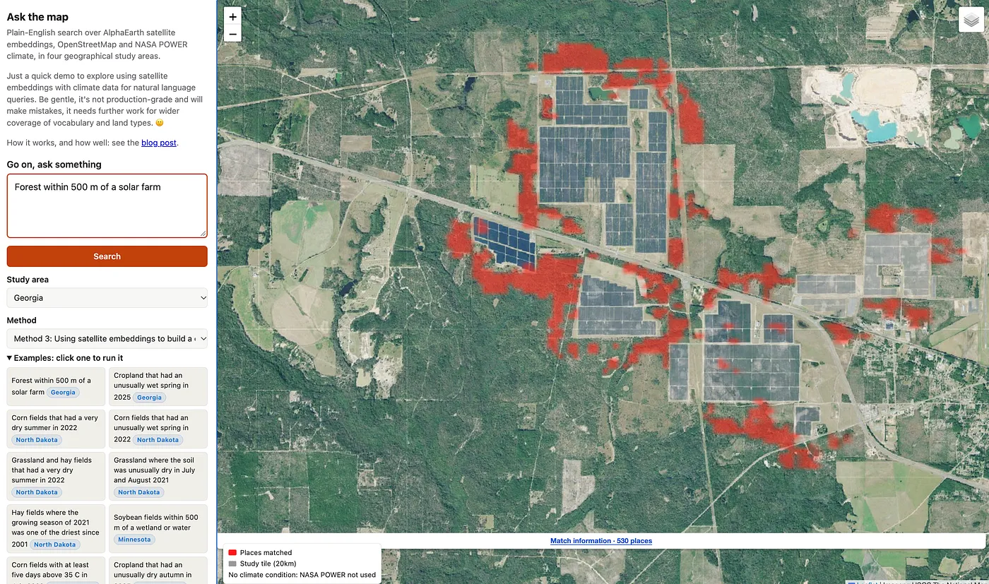
You can try the demo (to save costs it may take 30 seconds to wake up first time), and the code is on GitHub.
The Challenge
NASA POWER provides free solar and meteorological data for anywhere on Earth going back over 40 years, with more than 16 million requests from 50,000 unique users a month. People use it to design solar installations, model building energy use, and drive crop models, among many other things.
In a previous blog post, we explored using natural language queries for accessing this data, and since then NASA has said it is developing an AI agent and an MCP server for POWER, so AI platforms like ChatGPT and Claude could use this data directly.
That got me thinking …
Climate data alone is only half the story. What about questions that mix climate with what is on the ground?
- A crop insurance analyst: “Which corn fields had a heatwave during pollination?”
- A conservation officer: “Where is cropland right up against wetlands, where there has been high rainfall?”
- A solar developer: “Grassland near existing solar farms, in the sunnier part of the region.”
Normally, that means downloading climate grids, finding a land cover map, writing GIS code, and gluing it all together.
Instead, can we use natural language queries to find places in satellite maps and climate data?
Fingerprints for Places — Satellite Embeddings
Last year Google DeepMind released AlphaEarth Foundations, and with it a free dataset of satellite embeddings: for every 10m square of land, every year, a list of 64 numbers summarizing what the satellites saw over a year-long period. Fields with similar crops end up with similar numbers, wetlands look like other wetlands, and so on. Embedding meaning like this has been around for text - it’s a big part of internet search engines - but its application to satellite data is relatively new.
The catch is that these fingerprints are not directly related to natural language. You can’t type “wetlands” and get satellite images of wetlands back, it requires some work to link query language with the satellite embeddings.
There’s been some research on this, most recently AETHER (Tijūnaitytė et al., preprint), which aligns AlphaEarth embeddings and text embeddings using an approach similar to OpenAI’s CLIP, used for searching images. We will use this as inspiration in this article.
Side Note: Other work worth checking out includes Earth Genome’s Earth Index (search by labeled examples, with plain-language requests turned into OpenStreetMap tags), Google’s Earth AI agent (early access, plans over Google’s models including AlphaEarth) and BEACON (AlphaEarth embeddings aligned with point-of-interest text).
Ask the Map Prototype — Three Methods
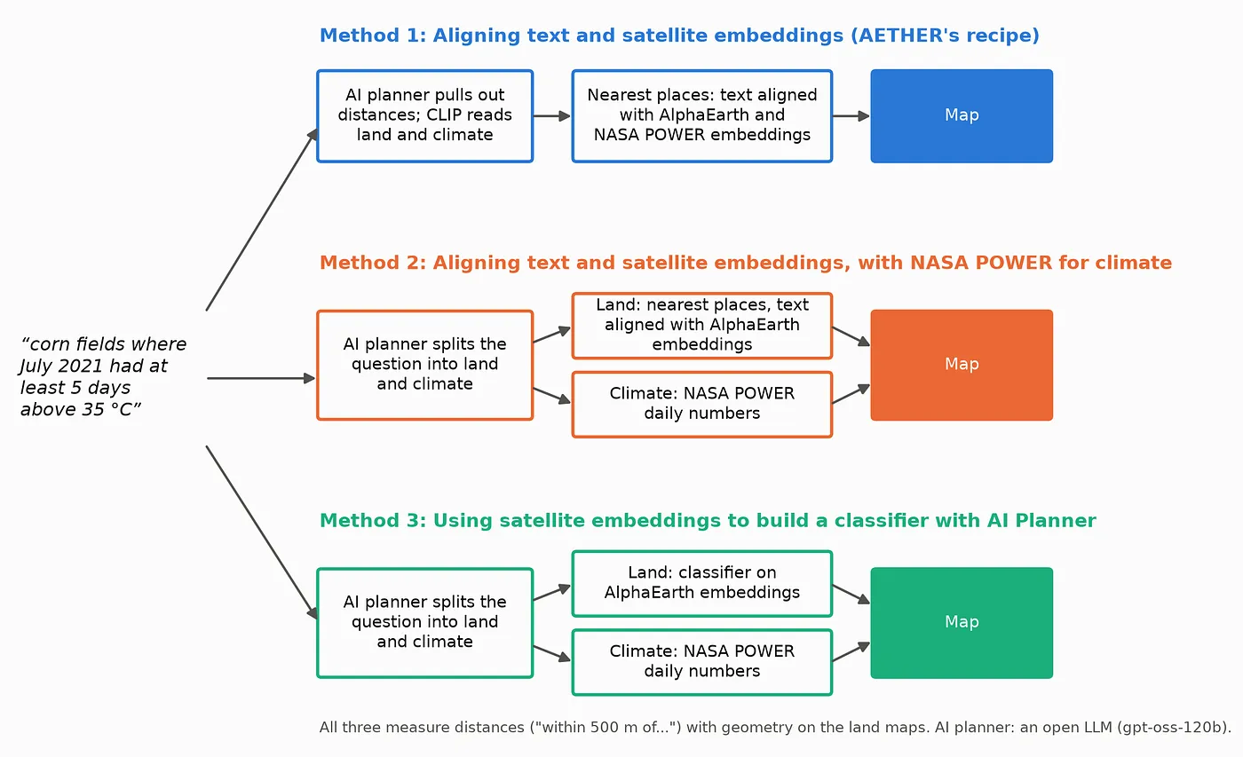
We’ll compare three methods which all start with an open LLM (OpenAI’s gpt-oss-120b via Hugging Face), which we’ll call the AI planner, turns the question into a small structured plan saying which land types, how near to what, and which climate conditions (see example plan below).
Then …
Method 1: Aligning text and satellite embeddings (AETHER’s recipe)
A small network was trained so that each location’s AlphaEarth embedding (plus a summary of its NASA POWER climate) lands close to text describing it. I automatically generated 510,930 captions (296,242 different ones) for 85,000 locations from the USDA Cropland Data Layer, the National Wetlands Inventory, the US Large-Scale Solar Photovoltaic Database, OpenStreetMap tags, and climate facts that I computed from NASA POWER’s daily data and worded myself, such as “where April-June 2022 rainfall was in the wettest 20% of years since 2001” (POWER supplies numbers, not sentences). Each caption is built by filling sentence templates with the facts known for that location (its crop or land type, whether a wetland, water, or solar farm is within a set distance, its OpenStreetMap tags, and its NASA POWER climate facts), so each location gets about six different captions. To answer a question, we embed the land and climate parts of it and return the nearest locations that also pass any distance rule. Elegant, one model, almost no rules. In AETHER’s pure form, the distances go in as words too, which is also scored below as a reference point.
Method 2: Aligning text and satellite embeddings, with NASA POWER for climate
The same aligned embeddings as Method 1, but with the climate removed from the text: only the land part of the plan goes through the aligned embeddings, and each climate condition is checked against NASA POWER’s actual daily data (see below).
Method 3: Using satellite embeddings to build a classifier with AI Planner
Each land type in the plan is found with a small model trained on AlphaEarth embeddings: a multinomial logistic regression over the 16 land types, which takes a pixel’s 64 AlphaEarth numbers plus the average and spread of its surroundings (150 m and 450 m windows) and gives it the most likely class. It is trained on 500,000 pixels sampled in their natural proportions from the training tiles, labeled by the official maps (USDA’s crop layer, the wetlands inventory and the solar farm database). Each climate condition is checked against NASA POWER’s daily data in the same way as Method 2.
For distances mentioned in queries, each method needs a land map to measure from. Method 3 uses its classifier. For Methods 1 and 2 we give every 30m patch whichever of 16 fixed land phrases (“corn fields”, “wetlands”, “existing solar farms” and so on) its aligned embedding is closest to, with no special rules for any land type. “Within 500 m of a solar farm” then means within 500 m of a patch on that map. When the question asks for something with no land type of its own (“a quarry”, “a golf course”, “barns”), Methods 1 and 2 use the question’s own words instead: the places whose aligned embedding sits closest to that phrase, with the “how many places” control on the page deciding how many. This approach is fairly basic, and certainly something that could be refined in future.
For example, “corn fields where July 2021 had at least 5 days above 35 °C” becomes …
{
  "land": {"classes": ["corn"]},
  "climate": [{"variable": "T2M_MAX", "years": [2021, 2021], "months": [7],
               "stat": "days_above", "day_threshold": 35,
               "test": {"kind": "absolute", "op": ">=", "value": 5}}]
}
Finally, to keep this quick, I chose a handful of 20 km study tiles rather than whole states: 45 of them across nine US states for training and scoring, and twelve (three in each of North Dakota, North Carolina, Minnesota and Georgia) in the demo.
How climate works in Methods 2 and 3
In Methods 2 and 3, the embeddings handle only the land. The AI planner turns each climate condition into a query of NASA POWER’s daily data:
- What to measure: a POWER variable (daily maximum temperature, rainfall, soil moisture, wind, humidity, sunlight, growing degree days), the months and years, and a statistic: an average, a total, or a count of days above or below a value.
- What counts as a match: a fixed threshold (“at least 5 days above 35 °C”), the place’s own history (“one of the wettest 10% of springs since 2001”), or the rest of the study area (“the sunnier half”).
- One answer per POWER cell: POWER’s grid cells are about 50 km across. For each cell over the study area we compute the statistic from the daily values and test it; for a history comparison the threshold is that cell’s own wettest (or driest, hottest…) 10% of years.
- Land and climate combined: every 30 m patch takes its POWER cell’s result, and a place is shown only if it is the right kind of land, passes any distance rule, and sits in a cell that meets every climate condition.
For the corn question above, the four North Dakota cells had 7, 7, 9 and 10 days above 35 °C in July 2021, so all pass and every corn field the classifier finds is shown. For “cropland where spring 2022 was one of the wettest 10% since 2001”, one cell had 299 mm of rain from March to May, compared with 220 mm in its own wettest 10% of springs, so we show the cropland in it. Because cells are so large, a condition tends to pass or fail for big chunks of a study area at once.
How Well Does It Work?
Using Claude Code I generated 58 questions in the style of real users: NASA POWER’s solar, building and agriculture communities, as well as USDA programs for crop insurance, drought payments and wetland conservation. Each one has an answer key computed from official maps (USDA’s crop map, the wetlands inventory and the solar farm database) plus POWER’s data. Pass marks were set before running anything, and the models were scored on states they never saw in training (Minnesota and Georgia, after training in the Dakotas, Nebraska, Kansas, Virginia and the Carolinas). In those states, 18 of the 58 have no right answer at all (nothing in the held-out study tiles meets them), so the held-out results use the other 40. Each question’s score is the F1 of its top-ranked places, taking as many places as the answer key has.
The headline results …
- The LLM understands the questions. Turning questions into plans scored a median F1 of 1.00 against hand-written plans, including reworded questions. A model small enough to run on a laptop (gpt-oss-20b) did just as well as the big one. Only 4 of the 58 questions tripped it up.
- Distances need geometry. My first versions of Methods 1 and 2 read distances as words, like the rest of the question, and on the 20 held-out questions with a distance rule they scored a median F1 of just 0.07 and 0.14. Measuring the distances with geometry instead lifted both to 0.45. Over all 40 held-out questions, Method 1 went from 0.23 (everything as words, as in AETHER’s design) to 0.48, and Method 2 from 0.49 to 0.58. Writing the plan back as text without the geometry barely helped (0.26), so it is the geometry that matters.
- Climate needs the numbers. For the 23 questions with a climate condition, Method 2 scored an average precision of 0.64 and Method 3 0.78, against 0.46 for Method 1, which embedded climate descriptions as text. This isn’t a huge surprise of course, embedding will lose some fidelity compared to a direct data query.
- With both fixes, Methods 2 and 3 are level. Method 2 scored a median F1 of 0.58 and Method 3 0.56 (0.64 with the improved land model in the next section), a gap well inside the noise of the comparison (its 95% interval runs from -0.15 to +0.11).
- The embeddings do know about common land types. The shared space’s own land map, where each patch takes the nearest land phrase, matched the official maps well for common land types (F1 0.91 for corn, 0.87 for soybeans, 0.84 for water, 0.79 for forest) but poorly for rare ones (0.42 for solar farms, 0.24 for spring wheat). And a simple test showed AlphaEarth has a clear wetland signal: averaging the embeddings of known wetlands and searching for similar pixels found wetlands at 6 to 8 times chance in North Dakota.
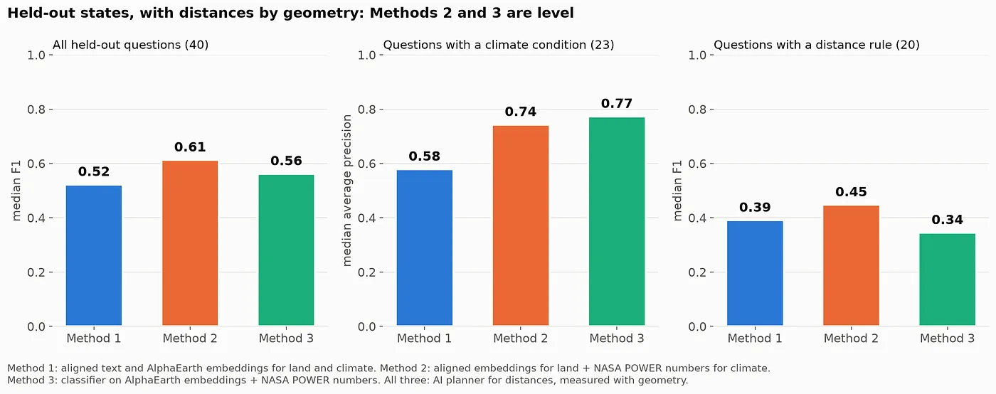
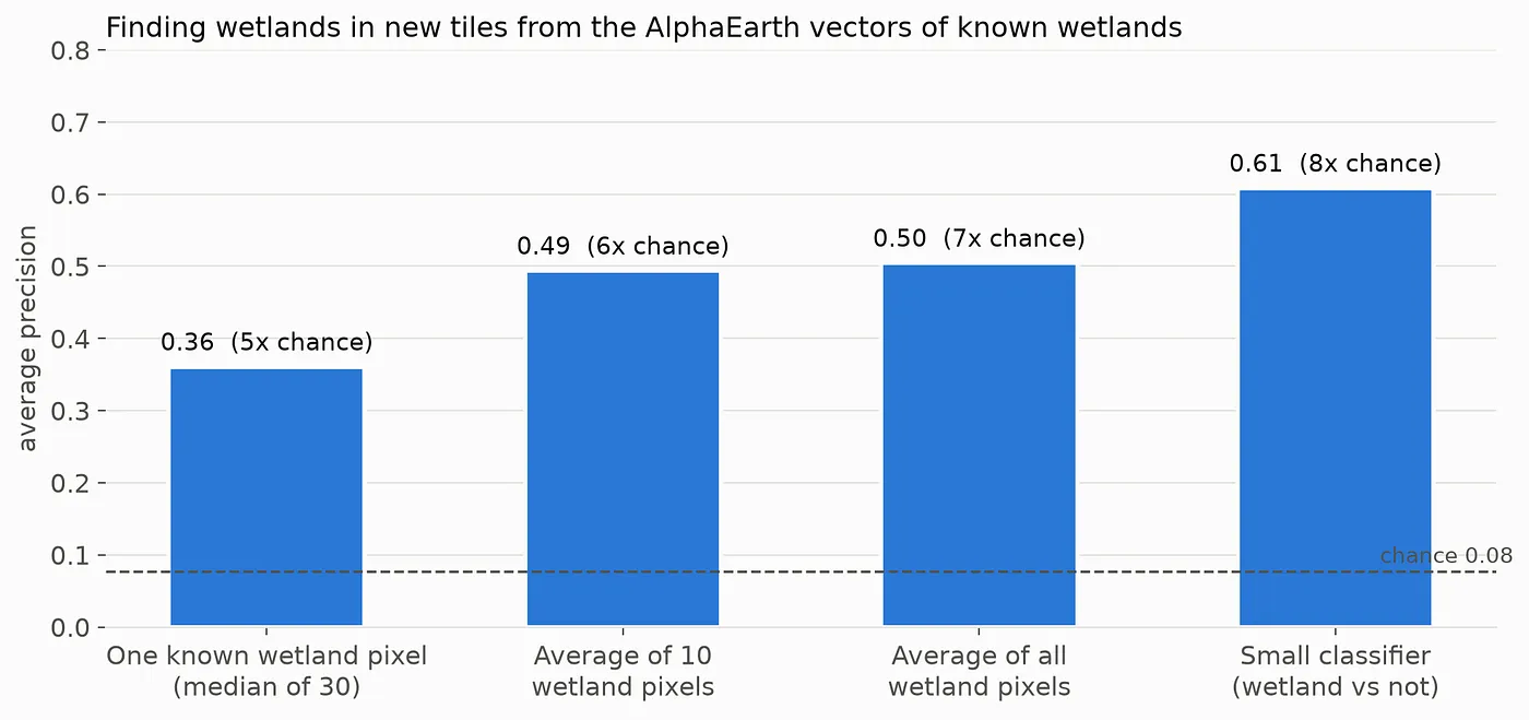
So the embeddings carry sufficient information, used for what it’s good at, recognizing land from a phrase, the shared space holds its own against a purpose-built classifier.
Super cool!
Fixing the False Alarms Without Special Rules
My first version of Method 3 used a separate yes/no detector for each land type, each trained on equal numbers of examples and non-examples. That worked for common things like corn, but it badly over-counted rare ones. In the Georgia test area, it marked 3,244 patches (90 m squares) as solar farms, where the official solar farm database has 919, so questions like “forest within 500 m of a solar farm” lit up forest next to solar farms that don’t exist.
The tempting fix is a pile of special rules (“solar farms must be at least 5 hectares”, “be stricter about wetlands”). To avoid hacks like that which are difficult to maintain, two general fixes that treat every land type the same way were tested instead: correcting each detector for how common its land type really is, and replacing the detectors with one model in which the land types compete, so a pixel is only called a solar farm if that beats forest, grassland and everything else. The second one won clearly on the held-out states …
- The average accuracy of the land maps (F1 over 14 land types) rose from 0.55 to 0.67.
- The median F1 over the 40 scored test questions rose from 0.47 to 0.71.
- In Georgia, the “solar farm” patches fell from 3,244 to 484. Across the held-out states, 99% of the patches it calls solar farms really are. It now misses some real ones, but it rarely invents them.
I then tried two more general improvements: letting the model see each place’s surroundings (the average embedding of the area around it, not just its own 30 m spot), and more training data (16 extra 20 km tiles, half of them centered on solar farms). Together they lifted the land maps a little further (F1 0.67 to 0.68) and solar farms noticeably (0.50 to 0.59), and “forest within 500 m of a solar farm” in Georgia went from an F1 of 0.44 to 0.61. That fell short of the +0.02 improvement set as the bar beforehand, but it mapped solar farms much better, so the demo uses it anyway.
Does Method 1 Understand Any Word?
Though the classifier performs better than the shared embedding space approach, it has the limitation of being trained on a fixed set of words. One of the selling points of aligning text and satellite embeddings (Methods 1 and 2) is that you should be able to type anything, not just the land types it was trained on. So I tested 17 words it never saw in training, using OpenStreetMap features in the study areas as the answer key, and compared them with 23 OpenStreetMap tags it was trained on.
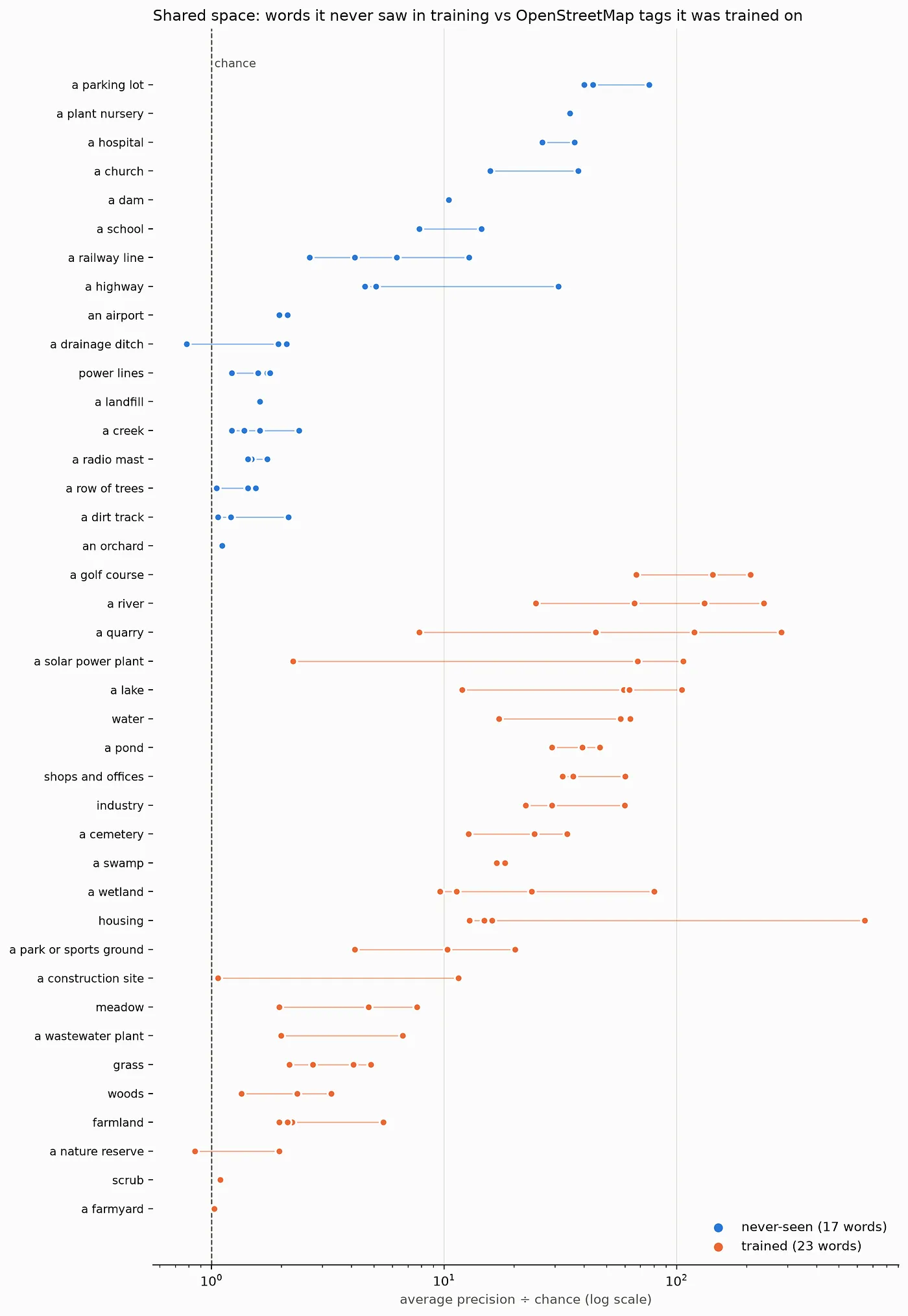
The answer is, well, “a bit”.
Never-seen words found the right places at a median of 1.9 times the chance, against 20 times the chance for trained tags. Built-up features did best (plant nurseries, churches, parking lots, hospitals and schools), while rural features like dirt tracks, rows of trees, creeks, drainage ditches, radio masts and power lines were barely better than chance. A likely reason is that the built-up words sit close in meaning to trained words like “housing” and “shops and offices”, though this hasn’t been checked. So “type anything” works for some things, but it is not a replacement for real training data in this work.
I also tried retraining the shared space to make it better: with a bigger vocabulary (three more OpenStreetMap tags, plus the LLM writing new wordings for every caption phrase), with each place’s surroundings, and with both. None of them cleared the bar set beforehand. Never-seen words stayed at 1.9 to 2.0 times the chance, whatever was tried (a fresh run of the original recipe gave 1.9). Looking at the LLM’s rewordings, quality was mixed (corn fields became “sweet corn acreage” and “corn belt fields”), which may explain why the bigger vocabulary did not help. On the 40 held-out questions, Method 2 moved between 0.54 and 0.58 across all five models, including a plain retraining of the original recipe (0.57 against 0.58), so these differences are no bigger than the noise between two training runs, and the demo keeps the original.
The Demo
You can try things out yourself in a simple demo app (it sleeps when nobody is using it — to save me money! — so the first visit after a quiet spell may take a minute or so to wake up). Type a question (or pick one of the examples), choose one of four study areas (North Dakota, North Carolina, Minnesota and Georgia), and the places that meet every part of the question light up on a satellite map. The NASA POWER grid cells behind any climate condition are drawn too: green where the condition holds, shaded where it doesn’t.
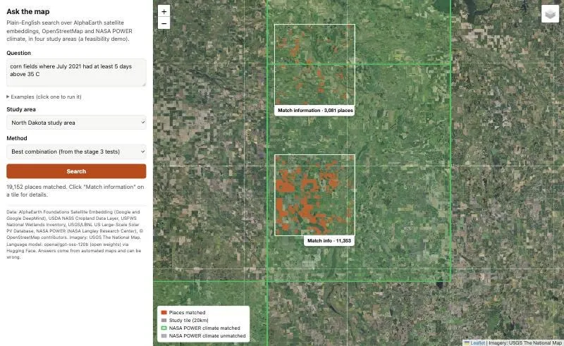
Each study tile has a Match information tab that opens the details for that tile: the question, what the LLM understood it to mean, how much land matched, the official land cover of the places shown, and, when the question involves climate, the actual NASA POWER values for each grid cell against the threshold.
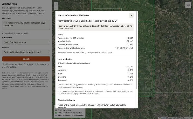
To check the answers properly, I scored the demo’s results for a few example questions against an answer key computed from the official maps and POWER’s data …
- “Corn fields where July 2021 had at least 5 days above 35 °C” in North Dakota: 93% of the places shown are correct, and it finds 94% of the right ones. 2021 was a scorcher there, with 7 to 10 such days in every POWER grid cell.
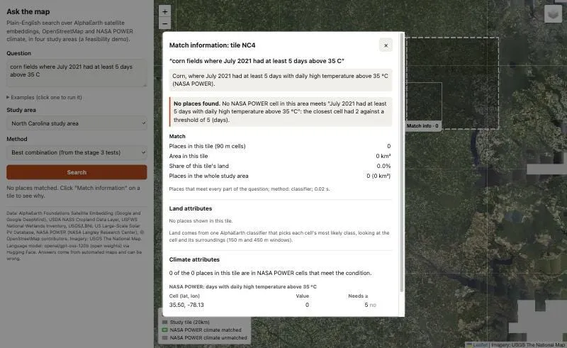
- The same question in North Carolina returns nothing, which is the right answer. The POWER cells there had 0, 0, 2 and 0 days above 35 °C that July, and the demo says so.
- “Grassland near an existing solar farm” in North Carolina is weaker: 42% of what it shows is correct. On the official map, 19% of what it shows is the solar farm itself, 14% is roads and farmsteads and 12% is forest. The reason isn’t pinned down yet, though grass between rows of panels looking like grassland to the satellites would be a good bet.
- “Wetlands next to crop fields” in North Dakota: 37% of what it shows is correct. On the official map 40% of it is wetland and a third is land the map leaves unclassified, so part of the gap is the answer key, not the demo. (“Next to” means the adjoining 90 m cell, a rule fixed after the LLM once read it as 30 m, finer than the grid, and returned nothing.)
Across the twelve example questions on the page, which were chosen because they work well, the ones that mix land with climate score an F1 of 0.72 to 0.94 with Method 3.
Limitations
It’s a quick prototype, so there are some important caveats …
- Accuracy drops in new places and for rare things. Even after the fixes, a median F1 of about 0.7 on held-out questions means roughly one place in three is wrong, and rare land types such as spring wheat in Minnesota are still poorly mapped.
- “Within X meters of something” questions are still the weakest. Even with geometry, the best method scores a median F1 of 0.45 on them in held-out states, and the demo’s examples of this kind score 0.61 to 0.72. In the one case traced in detail (forest near solar farms), the distances were right, and the errors came from the land map they were measured from, which had solar farms that don’t exist.
- Vague words are pinned down by rule, not by the LLM. Early on, asked the same question twice, the LLM once read “next to” as within 100 m and once as within 30 m, even with its randomness turned down to zero. The planner now has fixed rules (“next to” and “touching” mean adjoining cells, “near” means within 300 m, seasons have fixed months), and all twelve example questions give the same plan on three fresh calls. Other vague wordings may still wobble.
- The vocabulary is limited. Method 3 knows 16 land types. Methods 1 and 2 accept any phrase for land, but as shown above, words it never saw in training only work for some kinds of feature.
- Small study areas. The demo covers a few 20 km squares per state, not the whole country.
Future Work
The obvious next step is scale: the whole of the US, more land types, and the many other variables NASA POWER offers (solar, wind, humidity, soil moisture). The methods could also be fine tuned, for example analysis on how embeddings are combined could yield some improved results. It would also be fun to put this behind an MCP server, so you could ask Claude or ChatGPT these questions directly and get a map in response, which fits nicely with POWER’s own plans for an AI agent.
As always, I hope you found this interesting, and I’d love to hear from you!
Please follow me on Medium or LinkedIn for more noodling about with AI. 🙂
References
- NASA POWER Project, NASA Langley Research Center: power.larc.nasa.gov. “These data were obtained from the NASA Langley Research Center (LaRC) POWER Project funded through the NASA Earth Science/Applied Science Program.”
- NASA POWER usage (over 16 million requests from 50,000 unique users a month), NASA Technical Reports Server, May 2026: ntrs.nasa.gov/citations/20260004310
- NASA POWER 2025 Global Community Summit summary report: power.larc.nasa.gov/global-community-summit
- Harris, M. (2023). Creating a Climate GPT Using NASA’s Power API: medium.com
- Google DeepMind (2025). AlphaEarth Foundations helps map our planet in unprecedented detail: deepmind.google. The AlphaEarth Foundations Satellite Embedding dataset is produced by Google and Google DeepMind.
- Tijūnaitytė, van der Plas, Belaid, Knapen, Soja and Athanasiadis (2026). Domain-specific language alignment of multimodal embeddings towards explainable predictions (AETHER), arXiv preprint 2610.23110, version 1 posted 16 October 2026: arxiv.org/abs/2610.23110, code at github.com/WUR-AI/aether
- Tian, Cai and Yang (2026). BEACON: Behavioral and Semantic Enrichment of AlphaEarth Embeddings through Tri-Modal Contrastive Learning, arXiv 2608.29553 (accepted at ACM SIGSPATIAL 2026): arxiv.org/abs/2608.29553
- Koldunov and Jung, ClimSight (open-source climate decision-support tool): github.com/koldunovn/climsight
- cyanheads, nasa-power-mcp-server (community MCP server for NASA POWER, not a NASA product): github.com/cyanheads/nasa-power-mcp-server
- Radford et al. (2021). Learning Transferable Visual Models From Natural Language Supervision (CLIP), arXiv: arxiv.org/abs/2103.00020; OpenAI: openai.com/index/clip
- Earth Genome, Mapping the planet with Earth Index is now open to everyone (28 April 2026): earthgenome.org
- Earth Genome, Search for Stuff: build a map layer by describing what you want to find (29 September 2026): earthgenome.org
- Google Research, Putting Earth AI to work: Geospatial agents for our planet’s biggest challenges (14 October 2026): research.google
- Google Research, Google Earth AI: unlocking geospatial insights with foundation models and cross-modal reasoning (23 October 2025): research.google
- USDA National Agricultural Statistics Service, Cropland Data Layer 2024: nass.usda.gov
- U.S. Fish and Wildlife Service, National Wetlands Inventory: fws.gov
- USGS and LBNL, U.S. Large-Scale Solar Photovoltaic Database: energy.usgs.gov/uspvdb
- OpenStreetMap contributors, © OpenStreetMap, ODbL: openstreetmap.org/copyright
- OpenAI, gpt-oss-120b and gpt-oss-20b (open-weight models), via Hugging Face: huggingface.co/openai/gpt-oss-120b
Unless otherwise noted, all images are by the author.
You can try the demo (to save costs it may take 30 seconds to wake up first time), and the code is on GitHub.
Ask the Map: Finding Places Using Satellite Map Embeddings and NASA POWER Climate Data was originally published in AI Advances on Medium, where people are continuing the conversation by highlighting and responding to this story.